Stanford CS336 Day 11 - Parallelism 2

Howard · 2026年04月02日06:25

今日進度：8. Parallelism 2
今日花費時數：4

筆記

Building blocks of Distributed Communication/Computation

不論是單一 GPU 還是多 GPU 的 parallelism，都會遇到計算單元 (ALU) 離 inputs/outputs 相當遠的問題，因此我們的目標一直都是協調好計算流程來盡可能避免資料傳輸的瓶頸。在 Kernels, Triton 這個單元中，我們主要透過 fusion/tiling 等技巧來減少記憶體的存取次數，現在我們要透過 replication/sharding 來減少跨 GPU/Node 之間的通訊次數。

硬體通訊階層 (從快/小到慢/大)

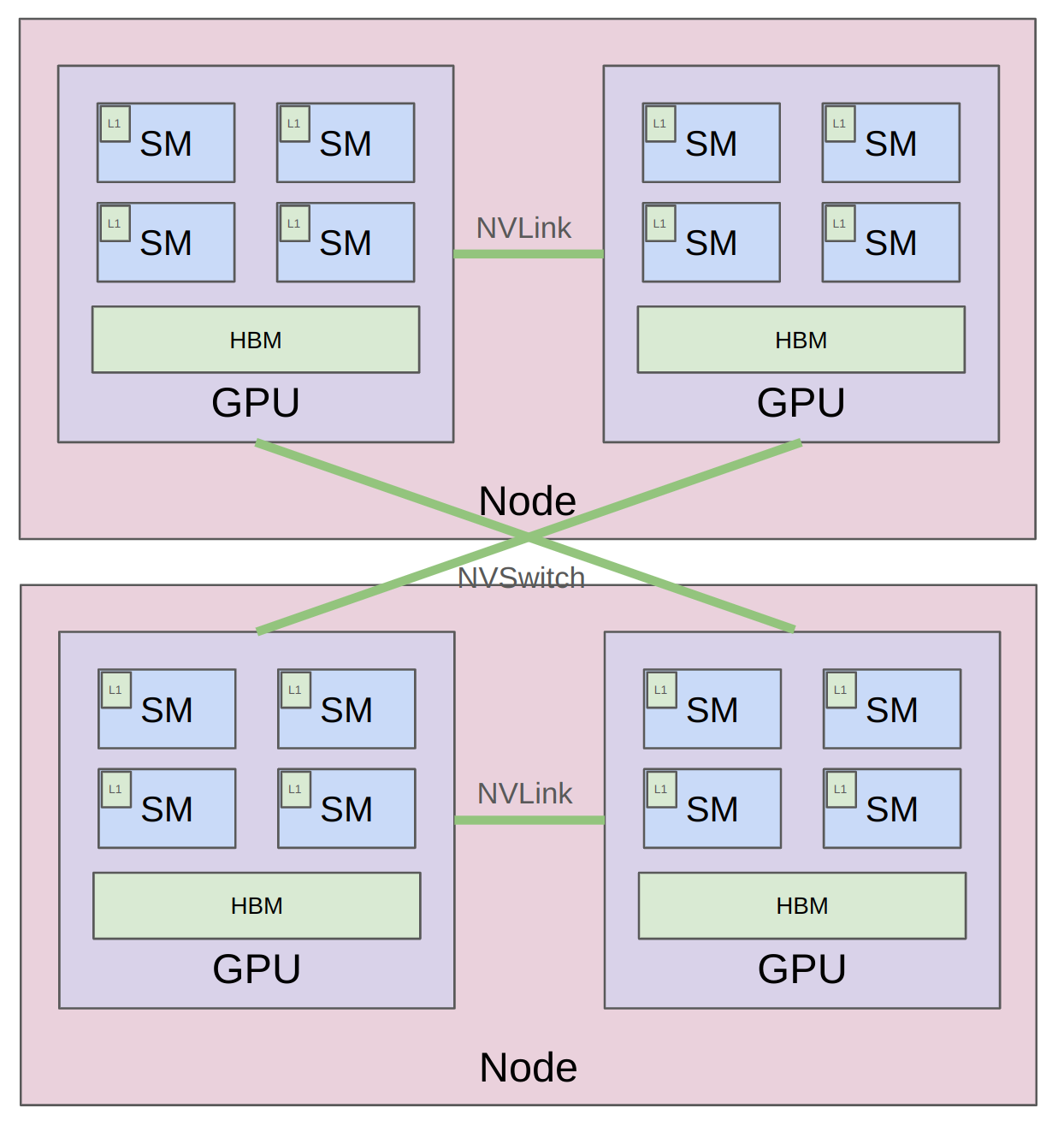
單一節點、單一 GPU：L1 cache/shared memory 速度極快但容量小，其次是高頻寬記憶體 (HBM)。
單一節點、多 GPU：現代資料中心使用 NVLink 直接連接 GPU，繞過傳統速度較慢的 PCIe 與 CPU 瓶頸。例如 H100 具備 18 個 NVLink 4.0 連接，總頻寬可達 900 GB/s。
跨節點、多 GPU：使用 NVSwitch 直接連接，繞過傳統且為非深度學習設計的乙太網路。

Collective Operations

首先我們要先來複習上一節課題教過的 collective operations, 這是一種針對多節點通訊的抽象化程式設計介面，比手動管理點對點通訊更有效率。

基本術語：

World Size：參與運算的總設備（GPU）數量。
Rank：設備的索引編號（例如 4 個設備的 rank 為 0, 1, 2, 3）。

Broadcast

將一個數值從單一 Rank 複製並傳送到所有其他 Rank。

Scatter

將一組不同的數值從單一 Rank 分別傳送到不同的 Rank 上。

Gather

Scatter 的反向操作，將來自不同 Rank 的數值收集到單一 Rank 上。

Reduce

類似 Gather，但在收集的同時會執行關聯/交換運算（如：加總、取最大/最小值）。

All-gather

與 Gather 相同，但將收集後的結果傳送到所有的 Rank 上。

Reduce-scatter

將各節點的數據進行 Reduce 運算後，把結果分散（Scatter）到不同的 Rank 上。

All-reduce = reduce-scatter + all-gather

這表示將所有節點的資料加總（或其他運算）並確保所有節點都獲得最終結果，其過程等同於先進行 Reduce-scatter 再進行 All-gather。

分散式硬體/軟體架構

1. 硬體連線架構

分散式訓練的通訊成本極高，因此硬體的演進一直致力於消除資料傳輸的瓶頸：

傳統架構

GPUs on same node communicate via a PCIe bus (v7.0, 16 lanes => 242 GB/s)
GPUs on different nodes communicate via Ethernet (~200 MB/s)
同節點通訊：GPU 之間透過 PCIe 匯流排溝通（例如 PCIe v7.0 頻寬約 242 GB/s）。缺點是資料傳輸時必須經過 CPU 與主機的內核，並複製到緩衝區，產生額外的負擔。
跨節點通訊：通常依賴乙太網路 (Ethernet)，傳輸速度相對極慢（約 200 MB/s）。乙太網路是很久以前設計的通用傳輸協定，並非為深度學習設計，因此會產生龐大的延遲。

現代資料中心架構 (NVIDIA 生態系)：

同節點通訊：使用 NVLink 直接將 GPU 串接在一起，完全繞過 CPU。以 NVIDIA H100 為例，每張卡具備 18 個 NVLink 4.0，總頻寬高達 900 GB/s。不過要注意的是，這個速度與 GPU 內部的高頻寬記憶體 (HBM, 頻寬約 3.9 TB/s) 相比，仍慢了約 4 倍左右。雖然 NVLink 讓 GPU 之間可以直接高速通訊並繞過 CPU，但系統中仍然需要保留 PCIe 匯流排，專門用來處理 CPU 與 GPU 之間的通訊。
跨節點通訊：使用 NVSwitch 直接連接不同節點的 GPU，直接繞過傳統的乙太網路，專為深度學習的運算負載進行最佳化。

硬體拓撲檢測：在 Linux 環境中，可以使用 nvidia-smi topo -m 指令來檢視 cluster 中 GPU 的連線狀態，例如確認 GPU 之間是否透過 NV18 連線，以及對應的網路卡設定。

2. 底層軟體：NCCL (NVIDIA Collective Communication Library)

擁有頂尖的硬體後，還需要軟體來驅動。NCCL 是 NVIDIA 提供的集合通訊函式庫：

指令轉譯：它負責將高階的集合運算指令（如 All-reduce）翻譯成 GPU 之間實際傳輸的底層封包。
自動最佳化：它會自動偵測硬體的拓撲結構（包含有幾個節點、Switch、NVLink 或 PCIe 的配置），幫你找出 GPU 之間最佳的資料傳輸路徑。
啟動運算：在規劃好路徑後，它會自動啟動 CUDA kernels 來進行資料的發送與接收。

3. 高階介面：PyTorch 分散式函式庫 (`torch.distributed`)

NCCL 對於一般開發者來說還是太底層了，而 PyTorch 則在 Python 層級封裝了這些複雜度：

乾淨的 API 介面：開發者只需寫一行程式碼（例如 dist.all_gather_into_tensor），PyTorch 就會幫你把 tensor 分發到不同 Rank 上。
支援多種硬體後端：
- nccl：專為 NVIDIA GPU 設計，提供最高效能。
- gloo：專為 CPU 設計的後端。這非常實用，代表即使在沒有 GPU 的筆電上，開發者也能用 CPU 模擬多個 Rank 進行分散式程式碼的開發與除錯，提高了程式的可移植性。
進階演算法封裝：torch.distributed 也支援像 FullyShardedDataParallel (FSDP) 這類更高階的演算法。

下面是一些關於 torch.distributed 使用方式的一些範例

import os
import torch
import torch.distributed as dist

def setup(rank: int, world_size: int):
    # Specify where master lives (rank 0), used to coordinate (actual data goes through NCCL)
    os.environ["MASTER_ADDR"] = "localhost"
    os.environ["MASTER_PORT"] = "15623"
    
    # Initialize the process group, choosing the backend based on hardware availability
    if torch.cuda.is_available():
        dist.init_process_group("nccl", rank=rank, world_size=world_size)
        
    else:
        dist.init_process_group("gloo", rank=rank, world_size=world_size)

上面這個 setup function 的目的是讓多個獨立的處理器能夠互相連結並形成一個工作群組。

行程協調連線：首先設定主節點的位址 (MASTER_ADDR) 與通訊埠 (MASTER_PORT)。這個連線僅是用來讓各個行程在啟動時互相找到彼此並進行基礎的「協調 (coordination)」。真正龐大的 tensor 資料傳輸，底層會自動交由 NCCL 處理。
自動切換後端：函式會自動偵測硬體環境，若有 GPU 則啟動專為 NVIDIA 最佳化的 nccl 後端；若無 GPU，則會切換成 gloo 後端，讓開發者可以用 CPU 來模擬多個 Rank 進行除錯，大幅提升了程式碼的方便性。

def collective_operations_main(rank: int, world_size: int):
    """This function is running asynchronously for each process (rank = 0, ..., world_size - 1)."""
    setup(rank, world_size)
    
    # All-reduce
    dist.barrier()  # Waits for all processes to get to this point (in this case, for print statements)
    
    # Create a unique tensor for each rank by adding the rank ID
    tensor = torch.tensor([0., 1, 2, 3], device=get_device(rank)) + rank  # Both input and output
    print(f"Rank {rank} [before all-reduce]: {tensor}", flush=True)
    
    # Sums the tensors across all ranks and stores the result back into each rank's tensor
    dist.all_reduce(tensor=tensor, op=dist.ReduceOp.SUM, async_op=False)  # Modifies tensor in place
    print(f"Rank {rank} [after all-reduce]: {tensor}", flush=True)
    
    # Reduce-scatter
    dist.barrier()
    
    # Create an input tensor of size equal to world_size
    input = torch.arange(world_size, dtype=torch.float32, device=get_device(rank)) + rank  # Input
    # Allocate a scalar (size 1) to hold the specific scattered chunk for this rank
    output = torch.empty(1, device=get_device(rank))  # Allocate output
    
    print(f"Rank {rank} [before reduce-scatter]: input = {input}, output = {output}", flush=True)
    
    # Performs a reduction (SUM) and scatters the results so each rank gets its corresponding chunk
    dist.reduce_scatter_tensor(output=output, input=input, op=dist.ReduceOp.SUM, async_op=False)
    print(f"Rank {rank} [after reduce-scatter]: input = {input}, output = {output}", flush=True)
    
    # All-gather
    dist.barrier()
    
    input = output  # Input is the output of reduce-scatter
    # Allocate an empty tensor of size world_size to collect the chunks back from all ranks
    output = torch.empty(world_size, device=get_device(rank))  # Allocate output
    
    print(f"Rank {rank} [before all-gather]: input = {input}, output = {output}", flush=True)
    
    # Gathers the individual chunks from all ranks and concatenates them into a complete tensor
    dist.all_gather_into_tensor(output_tensor=output, input_tensor=input, async_op=False)
    print(f"Rank {rank} [after all-gather]: input = {input}, output = {output}", flush=True)
    
    # Indeed, all-reduce = reduce-scatter + all-gather!
    torch.distributed.destroy_process_group()

這個 function 在所有設定好的行程中是非同步（Asynchronously）同時執行的。

同步點 (dist.barrier())：因為各行程的執行速度不一，dist.barrier() 就像一個檢查點，先抵達的行程必須停下來等待，直到所有人都到齊後才繼續執行。在此處主要目的是為了確保終端機輸出的 print 訊息能整齊排版，不會互相交疊。
All-reduce 操作：每張 GPU 建立好含有自身 rank ID 的張量後，透過 dist.all_reduce 將所有 GPU 上的 tensor 進行加總。這是一個 in-place operation，運算結果會直接覆寫原本的 tensor variable。
Reduce-scatter 操作：各 GPU 提供完整的 input tensor 並執行加總後，把結果「打散」，每張 GPU 最終只會被分配到屬於自己的一小部分（長度為 1 的 scalar），並存入預先宣告好的空白記憶體 output 中。
All-gather 操作：緊接著將剛剛 Reduce-scatter 算出來的「單一碎片」當作輸入，向全體發送 broadcast 並收集起來，最終在每張 GPU 上重新拼接出一個完整的 tensor。
資源清理 (torch.distributed.destroy_process_group())：這個指令的作用是安全地解散行程群組並進行資源清理 。當分散式運算任務執行完畢後，必須呼叫此函式來關閉在 setup 階段所建立的通訊連線，並釋放背後佔用的網路通訊與記憶體資源，確保程式乾淨地結束。

經過 All-gather 拼合後的結果，印出來會與最一開始執行 All-reduce 的結果完全相同，我們藉由實際執行證明了 All-reduce = Reduce-scatter + All-gather 的底層運算邏輯。

Benchmarking

class DisableDistributed:
    """Context manager that temporarily disables distributed functions (replaces with no-ops)"""
    def __enter__(self):
        self.old_functions = {}
        for name in dir(dist):
            value = getattr(dist, name, None)
            if isfunction(value):
                self.old_functions[name] = value
                setattr(dist, name, lambda *args, **kwargs: None)

    def __exit__(self, exc_type, exc_value, traceback):
        for name in self.old_functions:
            setattr(dist, name, self.old_functions[name])

def spawn(func: Callable, world_size: int, *args, **kwargs):
    # Note: assume kwargs are in the same order as what main needs
    if sys.gettrace():
        # If we're being traced, run the function directly, since we can't trace through mp.spawn
        with DisableDistributed():
            args = (0, world_size,) + args + tuple(kwargs.values())
            func(*args)
    else:
        args = (world_size,) + args + tuple(kwargs.values())
        mp.spawn(func, args=args, nprocs=world_size, join=True)

在評估分散式系統時，了解硬體實際的資料傳輸能力非常重要。以下程式碼展示了如何精確地測量 All-reduce 與 Reduce-scatter 的傳輸頻寬：

import time
import torch
import torch.distributed as dist

def benchmarking():
    # Let's see how fast communication happens (restrict to one node).
    # All-reduce
    spawn(all_reduce, world_size=4, num_elements=100 * 1024**2)
    
    # Reduce-scatter
    spawn(reduce_scatter, world_size=4, num_elements=100 * 1024**2)

def all_reduce(rank: int, world_size: int, num_elements: int):
    setup(rank, world_size)

    # Create tensor
    tensor = torch.randn(num_elements, device=get_device(rank))

    # Warmup
    dist.all_reduce(tensor=tensor, op=dist.ReduceOp.SUM, async_op=False)
    if torch.cuda.is_available():
        torch.cuda.synchronize()  # Wait for CUDA kernels to finish
        dist.barrier()            # Wait for all the processes to get here

    # Perform all-reduce
    start_time = time.time()
    dist.all_reduce(tensor=tensor, op=dist.ReduceOp.SUM, async_op=False)
    if torch.cuda.is_available():
        torch.cuda.synchronize()  # Wait for CUDA kernels to finish
        dist.barrier()            # Wait for all the processes to get here
    end_time = time.time()

    duration = end_time - start_time
    print(f"[all_reduce] Rank {rank}: all_reduce(world_size={world_size}, num_elements={num_elements}) took {render_duration(duration)}", flush=True)

    # Measure the effective bandwidth
    dist.barrier()
    size_bytes = tensor.element_size() * tensor.numel()
    sent_bytes = size_bytes * 2 * (world_size - 1)  # 2x because send input and receive output
    total_duration = world_size * duration
    bandwidth = sent_bytes / total_duration
    print(f"[all_reduce] Rank {rank}: all_reduce measured bandwidth = {round(bandwidth / 1024**3)} GB/s", flush=True)
		torch.distributed.destroy_process_group()

def reduce_scatter(rank: int, world_size: int, num_elements: int):
    setup(rank, world_size)

    # Create input and outputs
    input = torch.randn(world_size, num_elements, device=get_device(rank))  # Each rank has a matrix
    output = torch.empty(num_elements, device=get_device(rank))

    # Warmup
    dist.reduce_scatter_tensor(output=output, input=input, op=dist.ReduceOp.SUM, async_op=False)
    if torch.cuda.is_available():
        torch.cuda.synchronize()  # Wait for CUDA kerels to finish
        dist.barrier()            # Wait for all the processes to get here

    # Perform reduce-scatter
    start_time = time.time()
    dist.reduce_scatter_tensor(output=output, input=input, op=dist.ReduceOp.SUM, async_op=False)
    if torch.cuda.is_available():
        torch.cuda.synchronize()  # Wait for CUDA kerels to finish
        dist.barrier()            # Wait for all the processes to get here
    end_time = time.time()

    duration = end_time - start_time
    print(f"[reduce_scatter] Rank {rank}: reduce_scatter(world_size={world_size}, num_elements={num_elements}) took {render_duration(duration)}", flush=True)

    # Measure the effective bandwidth
    dist.barrier()
    data_bytes = input.element_size() * input.numel()  # How much data in the input
    sent_bytes = data_bytes * (world_size - 1)  # How much needs to be sent (no 2x here)
    total_duration = world_size * duration  # Total time for transmission
    bandwidth = sent_bytes / total_duration
    print(f"[reduce_scatter] Rank {rank}: reduce_scatter measured bandwidth = {round(bandwidth / 1024**3)} GB/s", flush=True)
    torch.distributed.destroy_process_group()

Warmup & Synchronization：在正式啟動計時器之前，我們必須先執行一次一模一樣的通訊操作來進行「暖身」。這麼做是為了確保所有需要的 CUDA kernels 都已經妥善載入。接著，必須呼叫 torch.cuda.synchronize() 等待 GPU 端運算完成，並呼叫 dist.barrier() 等待 CPU 端所有行程抵達同一點。這樣能保證程式碼量測到的是純粹的傳輸時間，而不會把系統啟動或行程等待的誤差時間算進去。
All-reduce 的頻寬計算：在計算 sent_bytes 時，All-reduce 的公式包含了一個 2 的係數。原因是 All-reduce 的運作牽涉到來回兩趟資料傳輸：每一個 Rank 都必須先送出自己的輸入資料到某個地方進行加總，然後還必須接收加總後的最終結果。因此，實際在網路中流動的資料量是單向傳輸的兩倍。
Reduce-scatter 的頻寬計算：在 Reduce-scatter 中，計算 sent_bytes 時則沒有 2 的係數。這是因為每個 Rank 只需要將自己的資料送出去進行加總，加總後的結果會直接打散（Scatter）並停留在對應的目標節點上。資料只會單向地收斂到各自的目的地，不會再被回傳給所有人，因此傳輸量減半。
測量結果與硬體理論值的差異：透過 bandwidth = sent_bytes / total_duration 算出的頻寬，即為實際的有效頻寬 (Effective Bandwidth)。在這節課的示範環境中，All-reduce 測出的頻寬大約為 277 GB/s。即使 H100 GPU 理論上具備總頻寬高達 900 GB/s 的 NVLink，但實際測量到的數值通常會低於理論上限，這取決於傳輸 tensor 的大小、節點數量，甚至底層 NCCL 的路徑最佳化狀況。因此，在實務開發時，親自撰寫這類 benchmarking 腳本來驗證系統效能是非常關鍵的步驟。

Distributed Training

Data Parallelism

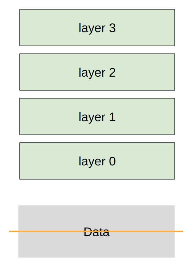
在 data parallelism 中，我們採取的 sharding strategy 是沿著 batch dimension 將資料切分，因此：

各個 rank 上的 loss 會彼此不同（用各自的 local data 計算）
梯度會在各個 rank 之間進行 all-reduce，使其保持一致
各個 rank 的模型參數會保持相同

def data_parallelism_main(rank: int, world_size: int, data: torch.Tensor, num_layers: int, num_steps: int):
    setup(rank, world_size)

    # Get the slice of data for this rank (in practice, each rank should load only its own data)
    batch_size = data.size(0)  # @inspect batch_size
    num_dim = data.size(1)  # @inspect num_dim
    local_batch_size = int_divide(batch_size, world_size)  # @inspect local_batch_size
    start_index = rank * local_batch_size  # @inspect start_index
    end_index = start_index + local_batch_size  # @inspect end_index
    data = data[start_index:end_index].to(get_device(rank))

    # Create MLP parameters params[0], ..., params[num_layers - 1] (each rank has all parameters)
    params = [get_init_params(num_dim, num_dim, rank) for i in range(num_layers)]
    optimizer = torch.optim.AdamW(params, lr=1e-3)  # Each rank has own optimizer state

    for step in range(num_steps):
        # Forward pass
        x = data
        for param in params:
            x = x @ param
            x = F.gelu(x)
        loss = x.square().mean()  # Loss function is average squared magnitude

        # Backward pass
        loss.backward()

        # Sync gradients across workers (only difference between standard training and DDP)
        for param in params:
            dist.all_reduce(tensor=param.grad, op=dist.ReduceOp.AVG, async_op=False)

        # Update parameters
        optimizer.step()

        print(f"[data_parallelism] Rank {rank}: step = {step}, loss = {loss.item()}, params = {[summarize_tensor(params[i]) for i in range(num_layers)]}", flush=True)

    torch.distributed.destroy_process_group()
    
data = generate_sample_data()
spawn(data_parallelism_main, world_size=4, data=data, num_layers=4, num_steps=1)

Data Slicing：程式碼首先獲取全部資料的 batch_size，接著將其除以 world_size 計算出 local_batch_size。每個 Rank 會根據自己的編號，計算出專屬的起始與結束 index，從中截取出屬於自己負責的那一小段批次資料，並將其傳送到對應的 GPU 上。
初始化完整的模型與優化器：這段訓練函式會在各個 Rank 上非同步（asynchronously）同時執行。因此，每個 Rank 都會獨立初始化一套完整的神經網路參數矩陣 (params)，以及建立屬於自己的 optimizer state。
前向傳播與損失計算：接著模型會如同標準的 SGD 一樣進行前向傳播與計算 loss。必須注意的是，因為每個 Rank 手上的訓練資料都是不同的，所以各個 Rank 所計算出來的 loss 也會不同。
核心關鍵：Sync Gradients：在執行完反向傳播 (loss.backward()) 後，真正的核心差異出現了。我們必須針對模型的每一層參數，呼叫 dist.all_reduce 並使用平均操作 (dist.ReduceOp.AVG) 來混合所有 Rank 算出的梯度。這個 all_reduce 操作同時也是一個同步點（synchronization point），會暫停跑得快的行程，確保所有的 Rank 都到齊並完成梯度平均後，才會繼續執行下一步。
一致的參數更新：由於先前的 all_reduce 已經將全體 Rank 的梯度平均化，因此此時所有 Rank 手上的梯度都是完全相同的。當最後各個 Rank 獨立呼叫 optimizer.step() 更新參數時，大家更新的幅度與方向就會一模一樣。這項機制保證了不管訓練幾步，所有 Rank 上的模型參數永遠都會保持完全一致。

Tensor Parallelism

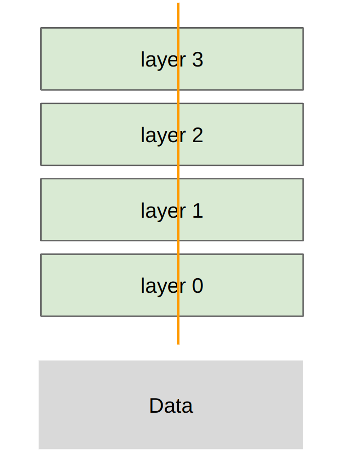
在 tensor parallelism 中，我們保留完整的訓練資料，將模型沿著「隱藏層維度/模型寬度 」進行切分。這代表每一個 GPU (Rank) 都會獲得完整的資料，但只會負責儲存與計算每一層神經網路的「一部分參數」。

def tensor_parallelism_main(rank: int, world_size: int, data: torch.Tensor, num_layers: int):
    setup(rank, world_size)

    data = data.to(get_device(rank))
    batch_size = data.size(0)  # @inspect batch_size
    num_dim = data.size(1)  # @inspect num_dim
    local_num_dim = int_divide(num_dim, world_size)  # Shard `num_dim`  @inspect local_num_dim

    # Create model (each rank gets 1/world_size of the parameters)
    params = [get_init_params(num_dim, local_num_dim, rank) for i in range(num_layers)]

    # Forward pass
    x = data
    for i in range(num_layers):
        # Compute activations (batch_size x local_num_dim)
        x = x @ params[i]  # Note: this is only on a slice of the parameters
        x = F.gelu(x)

        # Allocate memory for activations (world_size x batch_size x local_num_dim)
        activations = [torch.empty(batch_size, local_num_dim, device=get_device(rank)) for _ in range(world_size)]

        # Send activations via all gather
        dist.all_gather(tensor_list=activations, tensor=x, async_op=False)

        # Concatenate them to get batch_size x num_dim
        x = torch.cat(activations, dim=1)

    print(f"[tensor_parallelism] Rank {rank}: forward pass produced activations {summarize_tensor(x)}", flush=True)

    # Backward pass: homework exercise

    torch.distributed.destroy_process_group()
    
data = generate_sample_data()
spawn(data_parallelism_main, world_size=4, data=data, num_layers=4, num_steps=1)

Model Sharding：與 data parallelism 切割 batch_size 不同，這裡程式碼將隱藏層的維度 num_dim 除以 GPU 數量 (world_size)，計算出 local_num_dim。接著，每一層初始化的參數矩陣大小為 num_dim** * **local_num_dim**，這代表每個 GPU 只擁有整層神經網路參數的** *\frac{1}{\text{world size}}*。
Partial Activations：在前向傳播中，輸入 x 與當前 GPU 手上的那塊小參數矩陣 params[i] 相乘。算出來的結果 x 尺寸會縮小成 (batch_size, local_num_dim)，因為它只包含了該層「部分的」activations。
核心關鍵：All-gather & Concatenate：因為下一層的神經網路運算需要「完整」的輸入特徵，我們不能只拿著部分 activations 繼續往下算。因此，程式碼宣告了大小為 world_size 的 activations 列表，並呼叫 dist.all_gather。這個操作會向所有 GPU boardcast 收集各自算出的partial activations。收集完成後，使用 torch.cat(..., dim=1) 將它們接起來，重新還原成完整的 (batch_size, num_dim)，才能進入下一層的運算。
極高的通訊成本與硬體依賴：透過這段程式碼可以非常直觀地發現，在模型的「每一層」計算完畢後，都必須立刻進行一次龐大的 all_gather 資料傳輸。這種頻繁且大量的通訊特性，正是為什麼 tensor parallel 必須極度依賴如 NVLink 等高頻寬互連網路的原因，否則資料傳輸將嚴重拖垮整體訓練速度。

Pipeline Parallelism

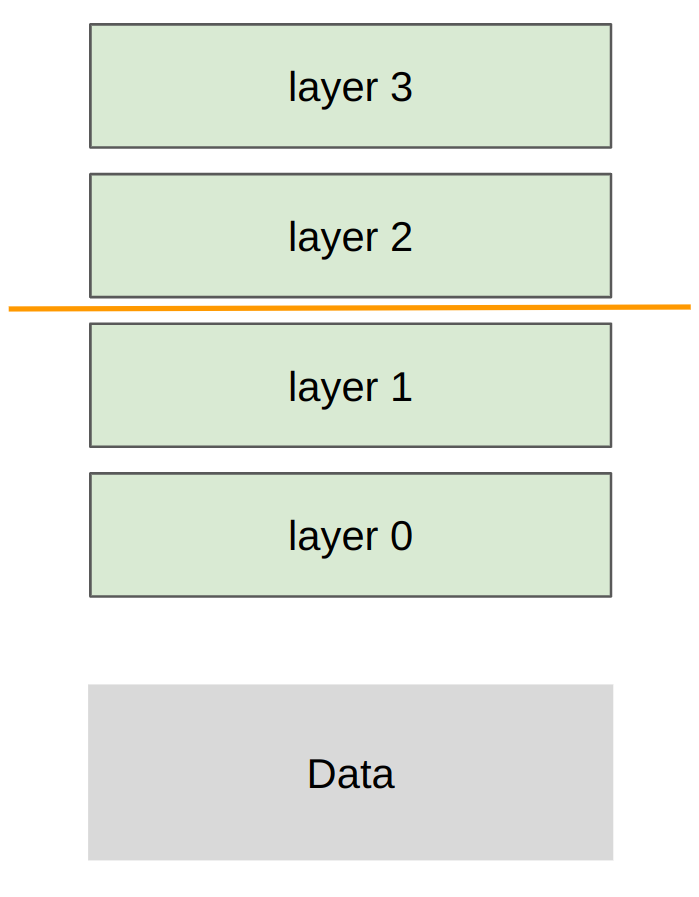
在 pipeline parallelism 中，我們採取的切分策略是將模型沿著「層數/深度維度」進行切分。這代表所有的資料都會依序進入 pipeline，但每一個 GPU (Rank) 都只會負責儲存並計算神經網路的「其中幾層」。

def pipeline_parallelism_main(rank: int, world_size: int, data: torch.Tensor, num_layers: int, num_micro_batches: int):
    setup(rank, world_size)

    # Use all the data
    data = data.to(get_device(rank))
    batch_size = data.size(0)  # @inspect batch_size
    num_dim = data.size(1)  # @inspect num_dim

    # Split up layers
    local_num_layers = int_divide(num_layers, world_size)  # @inspect local_num_layers

    # Each rank gets a subset of layers
    local_params = [get_init_params(num_dim, num_dim, rank) for i in range(local_num_layers)]

    # Forward pass

    # Break up into micro batches to minimize the bubble
    micro_batch_size = int_divide(batch_size, num_micro_batches)  # @inspect micro_batch_size
    if rank == 0:
        # The data
        micro_batches = data.chunk(chunks=num_micro_batches, dim=0)
    else:
        # Allocate memory for activations
        micro_batches = [torch.empty(micro_batch_size, num_dim, device=get_device(rank)) for _ in range(num_micro_batches)]

    for x in micro_batches:
        # Get activations from previous rank
        if rank - 1 >= 0:
            dist.recv(tensor=x, src=rank - 1)

        # Compute layers assigned to this rank
        for param in local_params:
            x = x @ param
            x = F.gelu(x)

        # Send to the next rank
        if rank + 1 < world_size:
            print(f"[pipeline_parallelism] Rank {rank}: sending {summarize_tensor(x)} to rank {rank + 1}", flush=True)
            dist.send(tensor=x, dst=rank + 1)

    text("Not handled: overlapping communication/computation to eliminate pipeline bubbles")

    # Backward pass: homework exercise

    torch.distributed.destroy_process_group()

data = generate_sample_data()
spawn(pipeline_parallelism_main, world_size=2, data=data, num_layers=4, num_micro_batches=4)

模型層數切分：與前面切分資料或切分隱藏層維度不同，這裡將總層數 num_layers 除以 GPU 數量 world_size，計算出 local_num_layers。每個 Rank 只會初始化分配給自己的那幾層參數。例如一個 4 層的網路分配給 2 個 GPU，Rank 0 就會負責前 2 層，Rank 1 則負責後 2 層。
核心關鍵：Micro-batches & Pipeline Bubbles： pipeline parallelism 最大的挑戰是「pipeline bubbles」：如果一次把整個 batch 餵進 Rank 0，下游的 Rank 1 在 Rank 0 算完之前都只能閒置等待。為了最大化硬體使用率，程式碼將原始的 batch 透過 data.chunk 切分成多個較小的 “micro-batches”。這樣一來，Rank 0 算完第一個 micro-batch 後，就能馬上傳給 Rank 1 處理，同時自己緊接著開始計算第二個 micro-batch。
點對點通訊 API (Point-to-Point Primitives)：在前兩種平行化策略中，我們都是依賴強大的 collective operations (如 all_reduce 或 all_gather)。但在 pipeline parallelism 中，資料是單向流動的，因此程式碼改用點對點通訊。
- dist.recv(tensor=x, src=rank - 1)：接收來自上一個節點 (上游) 計算完的激活值。
- dist.send(tensor=x, dst=rank + 1)：在自己負責的網路層計算完畢後，將結果直接傳送給下一個節點 (下游)。
未處理的進階最佳化：這段程式一個非常天真的基本實作，缺少了許多實務上需要的複雜邏輯。例如：
- 目前的 dist.send 與 dist.recv 是同步的，實務上應該使用非同步 (asynchronous) 操作來重疊「通訊」與「運算」的時間。
- 在加入反向傳播後，還必須精心安排並交錯執行 (interleave) 各個 micro-batch 的前向與反向運算順序（例如 1F1B 排程等），以保持 pipeline 的高效運作。

今日回顧與筆者的碎碎念

今天的內容主要是實作，因此內容總算沒有之前那麼艱澀難懂了，但要第二部分 systems 的部分完全融會貫通恐怕還要花費不少時間。不過好消息是 system 的部分總算結束了，接下來進入 scaling law 的部分，對筆者來說應該會輕鬆點吧？