本章由 Yeh 分享,筆記連結網址於此,由 Sky 取得同意後,整理如下。感謝 Yeh!
時間:2021年10月24日 20:00~20:20
與會人員:玉米, Shadow, Wayne, Yeh, Sky
分享:Yeh
646. Day 77 Goals: what you will make by the end of the day
- 電影預算和收入。
- 越高的電影預算會帶來越多票房收入嗎?
- 電影製片廠是否應在電影上花更多錢製作?
647. Explore and Clean the Data
- import/load data
import pandas as pd
import matplotlib.pyplot as plt

pd.options.display.float_format = '{:,.2f}'.format

from pandas.plotting import register_matplotlib_converters
register_matplotlib_converters()

data = pd.read_csv('cost_revenue_dirty.csv')
目標
- 資料集包含多少行和列?
- 是否存在任何NaN值?
- 是否有重複的行?
- 列的資料類型是什麼?
程式碼及輸出
- input1:
data.shape
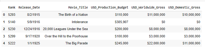
data.head()
- output1:
(5391, 6)
- input2:
data.isna().values.any() ##NAN
- output2:
False
- input3:
data.duplicated().values.any()
- output3:
False
- input4:
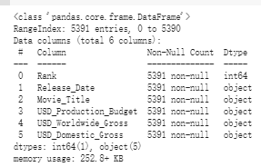
data.info()
- output4:
目標
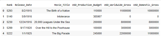
刪除 $ 和 , 符號,將 USD_Production_Budget 、USD_Worldwide_Gross 和USD_Domestic_Gross 列轉換為數字格式。
程式碼及輸出
- input1:
columns=["USD_Production_Budget","USD_Worldwide_Gross","USD_Domestic_Gross"]
for i in columns:
  data[i]=data[i].astype(str).str.replace(",","")
  data[i]=data[i].astype(str).str.replace("$","")
  data[i]=pd.to_numeric(data[i])
data.head()
- output1:
目標
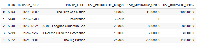
- 將
Release_Date列轉換為Pandas日期時間類型。
程式碼及輸出
- input1:
data.Release_Date=pd.to_datetime(data.Release_Date)
data.head()
- output1:
- input2:
data.info()
- output2:
<class 'pandas.core.frame.DataFrame'>
RangeIndex: 5391 entries, 0 to 5390
Data columns (total 6 columns):
 #   Column                 Non-Null Count  Dtype
---  ------                 --------------  -----
 0   Rank                   5391 non-null   int64
 1   Release_Date           5391 non-null   datetime64[ns]
 2   Movie_Title            5391 non-null   object
 3   USD_Production_Budget  5391 non-null   int64
 4   USD_Worldwide_Gross    5391 non-null   int64
 5   USD_Domestic_Gross     5391 non-null   int64
dtypes: datetime64[ns](1), int64(4), object(1)
memory usage: 252.8+ KB
648. Investigate the Films that had Zero Revenue
目標
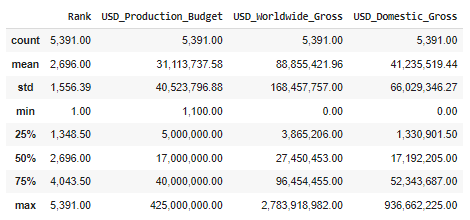
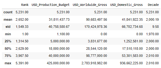
- 1.資料集中電影的平均製作預算是多少?31,113,737.58
- 2.全球電影的平均總收入是多少?88,855、421.96
- 3.全球和國內收入的最低限額是多少?0、0
- 4.最底層25%的電影實際上是盈利還是虧損?虧損
- 5.任何電影的最高製作預算和全球最高總收入是多少?425,000,000.00、2,783,918,982.00
- 6.最低和最高預算電影的收入是多少?1,100.00、425,000,000.00
程式碼及輸出
- input1:
data.describe()
- output1:
目標
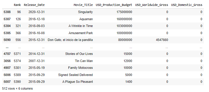
- 有多少部電影在國內(美國)的票房收入為0美元?什麼是沒有收入的最高預算電影?512、don gato el inicio de la pandilla
程式碼及輸出
- input1:
data[data["USD_Domestic_Gross"]==0].sort_values("USD_Production_Budget",ascending=False)
- output1:
**資料集編制日期2018年5月1日
目標
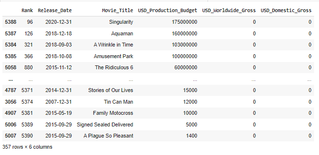
- 全球有多少電影票房為 0 美元?在國際上沒有收入的最高預算電影是什麼?357,The Ridiculous 6
程式碼及輸出
- input1:
data[data["USD_Worldwide_Gross"]==0].sort_values("USD_Production_Budget",ascending=False)
- output1:
649. Filter on Multiple Conditions: International Films
目標
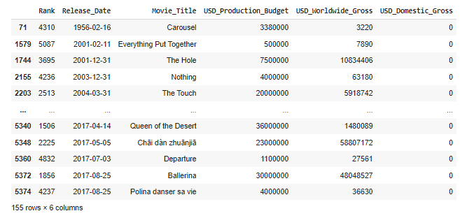
- 全球電影票房總收入但在美國零收入,創建一個子集。
程式碼及輸出
方法一:使用 .loc[]
- input1:
international_releases = data.loc[(data.USD_Domestic_Gross == 0) & (data.USD_Worldwide_Gross != 0)]
international_releases
- output1:
方法二:使用 .query() 。
- input1:
international_releases = data.query("USD_Domestic_Gross == 0 and USD_Worldwide_Gross != 0")
international_releases
- output1:
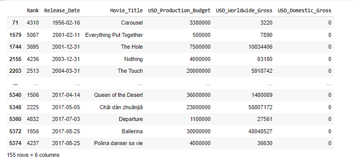
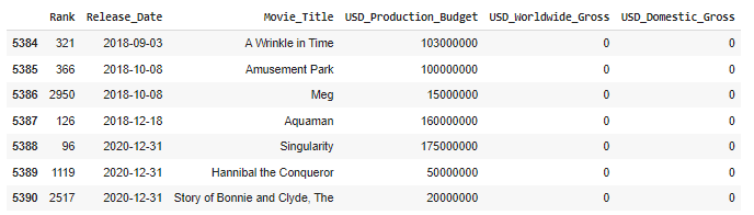
目標
- 截至數據收集時(2018年5月1日)哪些電影尚未上映。資料集中有多少電影還沒有機會在票房上映?(建立data_clean的dataframe)
程式碼及輸出
- input1:
# Date of Data Collection
after_scape_release=data[data.Release_Date>=scrape_date]
after_scape_release
# len(after_scape_release) #7
- output1:
- input2:
data_clean = data.drop(after_scape_release.index)
data_clean
- output2:
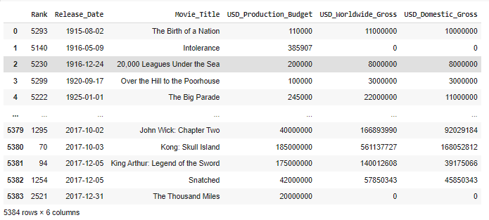
目標
- 製作成本超過全球總收入的電影百分比是多少?
程式碼及輸出
- input1:
data_money_lost= data_clean[data_clean.USD_Production_Budget>data_clean.USD_Worldwide_Gross]
data_money_lost
- output1:
- input2:
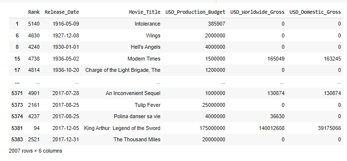
lost_percentage="{:.2%}".format(len(data_money_lost)/len(data_clean))
print(lost_percentage)
- output2:
37.28%
650. Seaborn Data Visualisation: Bubble Charts
目標
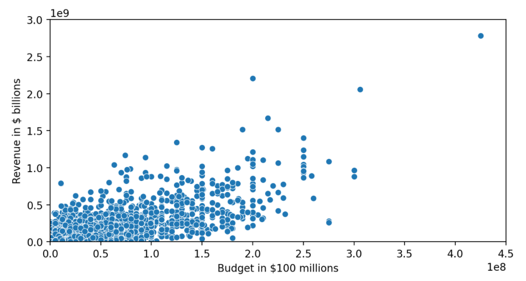
- 散佈圖
程式碼及輸出
- input1:
# Seaborn is built on top of Matplotlib
plt.figure(figsize=(8,4),dpi=200)
ax=sns.scatterplot(data=data_clean,x='USD_Production_Budget',y='USD_Worldwide_Gross')
ax.set(ylim=(0, 3000000000),xlim=(0, 450000000),
       ylabel='Revenue in $ billions',xlabel='Budget in $100 millions')
plt.show()
- output1:
目標
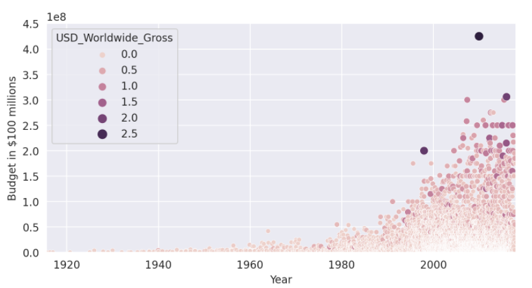
- 氣泡圖(bubble chart)
程式碼及輸出
- input1:
plt.figure(figsize=(8,4), dpi=200)

# set styling on a single chart
with sns.axes_style('darkgrid'): # style
  ax = sns.scatterplot(data=data_clean,
                       x='USD_Production_Budget',
                       y='USD_Worldwide_Gross',
                       hue='USD_Worldwide_Gross', #color
                       size='USD_Worldwide_Gross') #dot size

  ax.set(ylim=(0, 3000000000),
        xlim=(0, 450000000),
        ylabel='Revenue in $ billions',
        xlabel='Budget in $100 millions')
- output1:
651. Floor Division: A Trick to Convert Years to Decades
目標
- 單位:年轉換成十年
程式碼及輸出
- input1:
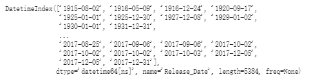
dt_index = pd.DatetimeIndex(data_clean.Release_Date) #Create a DatetimeIndex object
dt_index
- output1:
- input2:
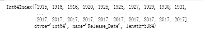
years = dt_index.year
years
- output2:
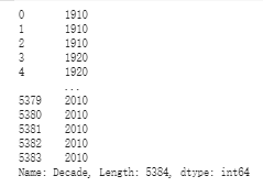
- input3:
data_clean['Decade']=years//10*10
data_clean.Decade
- output3:
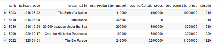
- input4:
data_clean.head()
- output4:
目標
- 依據1970年切割成2個dataframe
程式碼及輸出
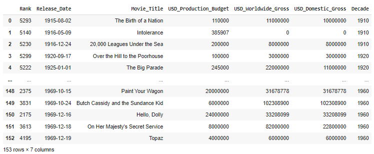
- input1:
before_data=data_clean[data_clean.Decade<1970]
before_data
- output1:
- input2:
after_data=data_clean[data_clean.Decade>=1970]
after_data
- output2:
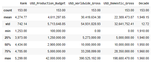
- input3:

before_data.describe()
- output3:
- input4:
after_data.describe()
- output4:
652. Plotting Linear Regressions with Seaborn
目標
- 線性回歸將電影預算與全球收入間的關係視覺化
.regplot() - Before 1970
程式碼及輸出
- input1:
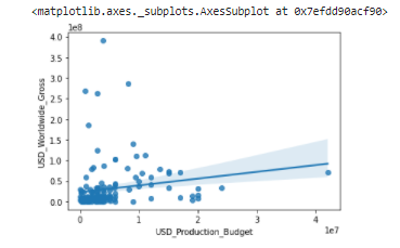
sns.regplot(data=before_data,
            x='USD_Production_Budget',
            y='USD_Worldwide_Gross')
- output1:
- input2:
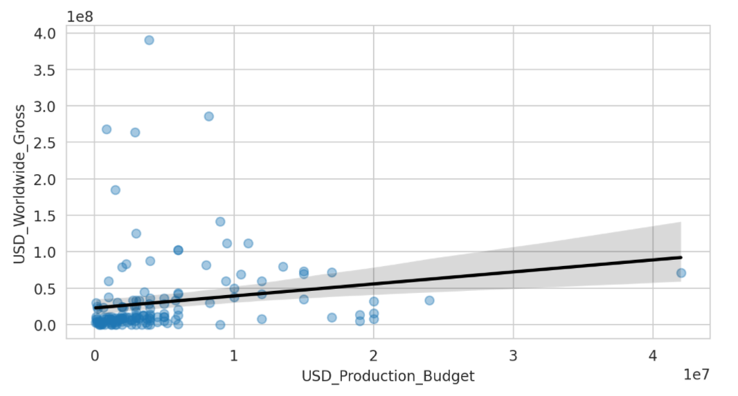
plt.figure(figsize=(8,4), dpi=200)
with sns.axes_style("whitegrid"): #grid
  sns.regplot(data=before_data,
            x='USD_Production_Budget',
            y='USD_Worldwide_Gross',
            scatter_kws = {'alpha': 0.4},
            line_kws = {'color': 'black'})
-
output2:
-
電影製作預算和電影收入之間的關係不強。
目標
- After 1970
程式碼及輸出
- input1:
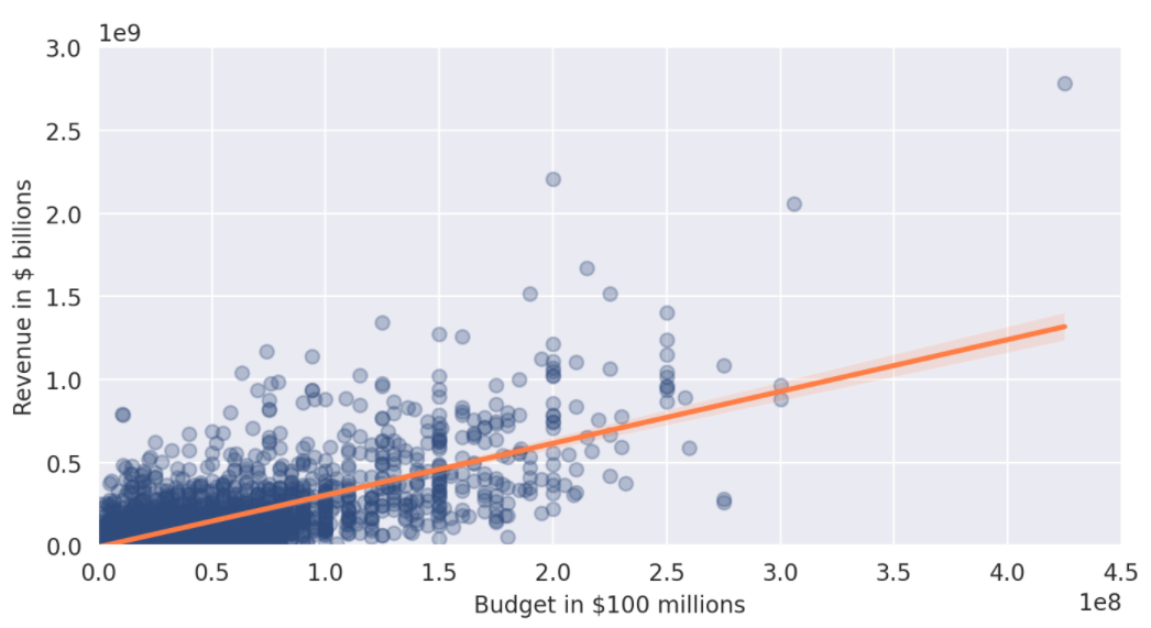
plt.figure(figsize=(8,4), dpi=200)
with sns.axes_style('darkgrid'):
  ax = sns.regplot(data=after_data,
                   x='USD_Production_Budget',
                   y='USD_Worldwide_Gross',
                   color='#2f4b7c',
                   scatter_kws = {'alpha': 0.3},
                   line_kws = {'color': '#ff7c43'})

  ax.set(ylim=(0, 3000000000),
         xlim=(0, 450000000),
         ylabel='Revenue in $ billions',
         xlabel='Budget in $100 millions')
- output1:
- 預算為1.5億美元的電影->約5億美元收入
653. Use scikit-learn to Run Your Own Regression
目標
- 使用scikit-learn線性回歸模型
- 找出模型對theta的估計值。
- 對
before_data運行線性回歸。計算截距、斜率和 r-squared。在這種情況下,線性模型可以解釋多少電影收入的差異?- y軸上截距:若預算為0電影的收入是多少。
- 斜率:電影預算增加1美元可獲得多少額外收入。
程式碼及輸出
- input1:
from sklearn.linear_model import LinearRegression
regression = LinearRegression()

# Explanatory Variable(s) or Feature(s)
X = pd.DataFrame(after_data, columns=['USD_Production_Budget'])

# Response Variable or Target
y = pd.DataFrame(after_data, columns=['USD_Worldwide_Gross'])

# Find the best-fit line
regression.fit(X, y)
- ouptut1:
LinearRegression(copy_X=True, fit_intercept=True, n_jobs=None, normalize=False)
- input2:
regression.intercept_ # theta 0
regression.coef_ # theta 1
- output2:
array([-8650768.00661027])
array([[3.12259592]])
-
預算每增加1美元,電影收入就會增加約3美元。
-
input1:
# R-squared
regression.score(X, y)
- output1:
- r-squared約為0.558。
- 模型解釋約56%的電影收入差異。
654. Learning Points & Summary
-
Use nested loops to remove unwanted characters from multiple columns
-
Filter Pandas DataFrames based on multiple conditions using both .loc[] and .query()
-
Create bubble charts using the Seaborn Library
-
Style Seaborn charts using the pre-built styles and by modifying Matplotlib parameters
-
Use floor division (i.e., integer division) to convert years to decades
-
Use Seaborn to superimpose a linear regressions over our data
-
Make a judgement if our regression is good or bad based on how well the model fits our data and the r-squared metric
-
Run regressions with scikit-learn and calculate the coefficients.